Linear Regression Part II
OLS Part 2
Regression Analysis
In the previous post we had a quick sneak peak into Regression and Ordinary Least Squares Regression in particular. In this post we will build onto those concepts and understand how a linear regression model is built and evaluated. We will use some python to get the job done!
Quick Refresh
Simple linear regression is an analysis of relationship between two variables, say x and y, which are linearly dependent (linear regression you see) they can be mathematically denoted as-
Y = a + b.X
where,
- Y: dependent variable
- X: independent variable
- a: intercept of the line
- b: slope of the line
Note: Going forward we will utilize the same Height-Weight data set from the previous post.
Sample Verses Population
While building the regression line from our Height-Weight data set we made use of the complete data set and also termed our regression line as the population regression line. But in a real world scenario, we might never have the complete population (all data points) to play with. How do we go about building a regression line in such a case?
Statistics and Data Science per say is the art of making best possible use of what you have. In most cases we have only a small subset of the complete data. This may be due to limitations in data collection processes, erroneous data or simply the data might not exist at all. So to form a regression line, we use this subset of data and follow the complete process. This process would give us some values for the slope and intercept of the regression line. Since we would use the values of slope and intercept from the sample to learn the parameters of the actual population, it should be noted that the values (of slope and intercept) might change if the sample itself changes. To ensure that the regression parameters of slope and intercept from the sample are good estimates of the population parameters, we make and observe the following assumptions:
-
The mean of dependent variable (
Y) is a linear function of each value of independent variableX. The regression line emulates the mean behavior of data. This is evident from the formulae derived to compute slope and intercept (see previous post). -
The error between the computed weight for a given height and the actual weight for each data point is independent of other data points in the data set. It is obvious that there will be error in the observed and the actual value of dependent variable. But the point that these errors are independent is important.
-
The probability distribution of sample errors is a normal distribution
-
The errors for independent variable X have equal variance.
Regression Evaluation : R-Squared
By now we know that we will have to deal with just a sample of the overall population in most cases to build a regression model. We also understand that each sample will generate a different regression line which would be off from the actual regression line within some error bounds. But how do we determine if our regression line is good at all or not?
The Coefficient of Determination or R-Squared as it is usually known, is a measure widely used to determine if the regression line is able to indicate the variance in the dependent variable as explained by the independent variable. To understand this better, we introduce 3 measures:
- Sum of Squares Explained (SSE): this is a measure of how much the data points vary from the regression line.
SSE = ∑(y - y_regression)²
- Regression Sum of Squares (SSR): this is a measure between the estimated regression line and the mean line (or line of no relationship).
SSR = ∑(y_regression - y¯)²
- Total Sum of Squares(TSS): this is a measure to denote the variance of data points around mean.
TSS = ∑(y - y¯)²
Note that TSS = SSE + SSR and we denote R-Squared as:
R² = SSR / TSS
i.e. R² points out to the fact that a regression line better represents the data if the total variance in data(TSS) is dominated by its regression variance(SSR). Since TSS is a sum of other two measures, R² is a real number between 0 and 1. The following are a few observations related to R²:
- R²=1 denotes that all points fall perfectly on the regression line, i.e. the independent variable is able to explain all the variation in the dependent variable.
- R²=0 denotes that independent variable is not able to explain the variance in the dependent variable. The regression line lies perfectly horizontal.
A higher value of R² (values closer to 1) points to the fact that the independent variable is able to explain (or is able to account for) the variance in the dependent variable.
This by no means refers to something like “the independent variable causes the changes in the dependent variable”. In our example, Height explains or accounts for the variation in Weight. It by no means implies that a certain Height causes a certain Weight.
Hands-On Time
Let us continue with our Height-Weight sample data set and see what kind of regression model we can build out of it. To begin with, we would be making use of some awesome python packages, namely:
-
pandas: for handling data in the form of data frames. This library provides some very useful utilities to analyze and handle data.
-
statsmodels: as the name suggests, it helps us with statistics, particularly regression for this post.
-
matplotlib: the de-facto plotting package.
Let’s get started with loading the data first:
df = pd.DataFrame.from_csv(r'data\student_height_weight.csv',
                           index_col=None)
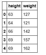
df.head()
The head() function helps us view a top few rows of the data. The sample data looks something like this:
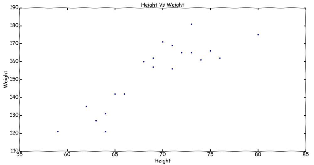
The same data on a plot looks like this:
Time to build an OLS model for the same. Using a package like statsmodels makes things really easy. All we need to do is prepare our independent and dependent variables from the data set and rest of the magic happens in a breeze. Remember, behind the scenes all the theory we covered is being used to get the final results.
# Set the independent variable
X = df1.height.values.tolist()

# This handles the intercept.
# Statsmodel takes 0 intercept by default
X = sm.add_constant(X)

# Set the dependent variable
y = df1.weight

# Build OLS model
model = sm.OLS(y, X)
results = model.fit()

# Get the predicted values for dependent variable
pred_y = results.predict(X)

# View Model stats
print(results.summary())
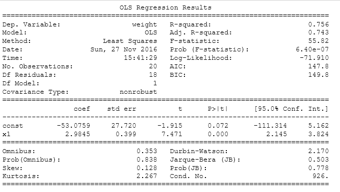
The OLS model’s summary is as follows:
Model Summary:
-
The above results present an intercept of -53.0759 and a slope of 2.9845.
-
A positive slope shows an upward trend.
-
R² of 0.756 points towards a good enough model, i.e. the height (independent variable) is able to explain 75.6% of variance in weight (dependent variable).
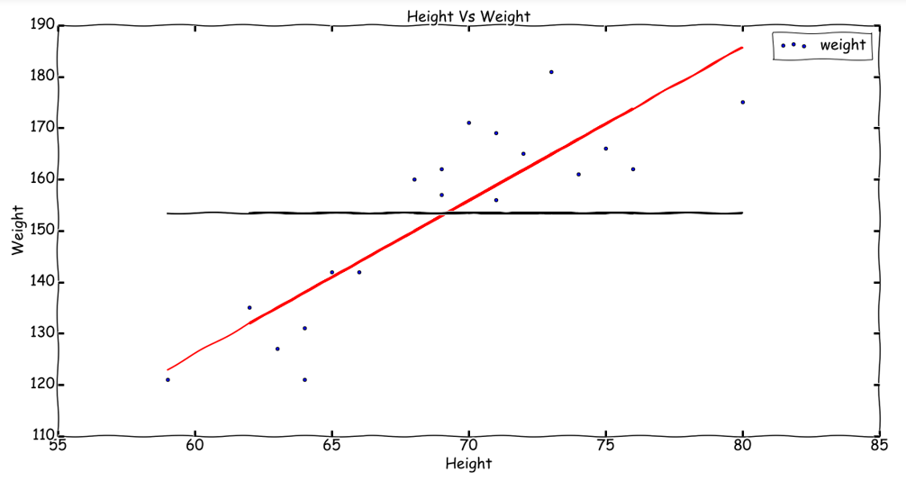
The final output can be visualized with a few lines of code:
# plot the data points
plt.scatter(df1.height,df1.weight)

# plot the regression line
plt.plot(df1.height,pred_y,color='red')

# plot the mean line
plt.plot(df1.height,
         [df1.weight.mean()]*df1.weight.count(),
         color='black')
The plot:
Conclusion
The second post in the linear regression series adds on to the concepts we learnt in the first post. We understood the concept of Coefficient of Determination or R-Squared along with a sample implementation of OLS in python using statsmodels package.
The complete notebook is available: python_notebook.


