Regression Analysis

It includes various techniques for modeling and analyzing these relationships. Regression Analysis has roots in statistics but is widely used in the machine learning space. It is used for predictive analysis, forecasting and time series analysis. Another use case for regression analysis is causal-effect relationship, though this should be considered with a pinch of salt.

Simple Linear Regression

Starting off with simple things, Simple Linear Regression is analysis of two continuous variables of which one is termed as dependent (or response) while the other is called independent (or predictor). Some examples of statistical relationship between two variables could be-

• Relationship between height and weight- The weight of a person increases with height, though not perfectly or always.
• Relationship between vehicular speed and number of accidents- The number of accidents are higher at higher speeds, though not always necessary.

Since simple linear regression is an analysis of relationship between two variables, say x and y, which are linearly dependent (linear regression you see) they can be mathematically denoted as-

Y = a + b.X

where,

• Y: dependent variable
• X: independent variable
• a: intercept of the line
• b: slope of the line

The Classic Height-Weight Example

As is the common perception, weight and height are related parameters for us humans. The taller you are the heavier you get (well, usually and not always :) ).

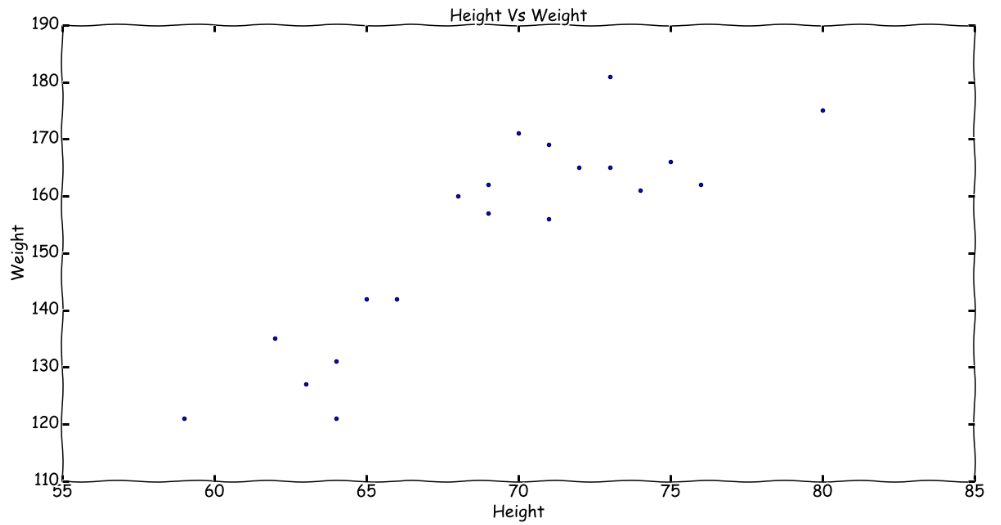
Continuing with our Height-Weight sample data set, let us apply some linear regression concepts. The data set contains the weight and height measurements of a certain imaginary population (these values have been generated randomly for demo purposes).

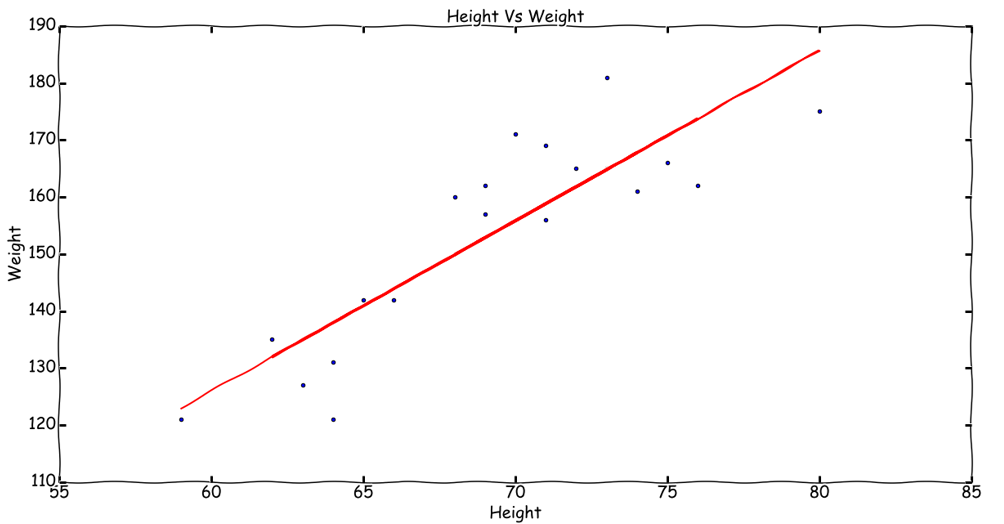
By now we know that Regression is the analysis of independent and dependent variables, in our current example, we have the variable weight which depends on height of a person. Thus, weight is dependent while height is independent. We could use this information to predict/guess the weight of a person whose height we know. To formalize this behavior, we can draw a line through the data points to depict this relationship. The relationship can be depicted as:

Weight = a + b.Height

We can obtain different lines for different settings of a and b. But now the question arises, which line represents the relationship most correctly? For what values of these variables will we be able to predict an unknown person’s weight given his/her height? Luckily, we have a few data points which we can utilize to get as close a prediction as possible.

The Best Fit

The line which best fits our Height-Weight relationship would require a bit of experimentation. Let us denote the data set containing height and weight of people as D, which contains data points in the form of (h,w) for each person. We also denote the set of all know heights as H and all known weights as W.

Now, the experiment can be designed as follows:

• Let us start with an arbitrary line. Say a line between the lowest point and the highest point in the scatter plot (least height-weight and max height-weight respectively). This particular line would have certain intercept and slope, i.e. a and b respectively.
• For this line we calculate weight for each person’s height we have in the set H. Let these set of weights be denoted as W'.
• Since we already have weights for all people in our dataset, we compare how off the weights inW' are with respect to W. Let this difference between observed and actual values of weights be denoted as error e.

Now, our notion of a best fitting line can be easily explained in terms of error e. The error between the observed and the actual is a clear indicator of how well we map the height-weight relationship. Now, how do we define and calculate the metric e ?

Calculating Errors

For starters we could begin with a simple difference between the observed and actual values. Such an error measure is termed as prediction error and denoted as:

e = w - w’

The best fitting line would have least prediction error for each data point in our data set. One problem with such an error measure is that it carries a sign. A signed measure has the probability of cancelling out when summed (can you visualize the issue here?).

To avoid this, we make use of sqaured prediction error, i.e.:

e² = (w-w’)²

To achieve the overall squared prediction error for a line in consideration, we use the least squares criterion i.e. the overall squared prediction error for a given line is sum of squared errors for each of its data points.

q = ∑(w-w’)²

Least Squares Estimates

We could go on repeating the experiment of picking up any arbitrary line and calculating its sqaured prediction error. But we also know that there could be an infinite number of lines and checking all of them is actually not possible. Then how do we arrive at our best fit?

Luckily finding that perfect fit would require certain values for its intercept and slope (a and b). Such a line would have least value for its overall squared error q, i.e. we need to simply minimize q with respect to a and b:

q = ∑(w-w’)²

=> q = ∑(w-(a+b.h))²

This involves a bit of a calculus and what we get as output is termed as the least squares regression line which would have least possible squared error! The intercept and slope are given as:

a = w¯ − bh¯

and

b = ∑(h−h¯)(w−w¯) / ∑(h−h¯)²

where:

• w¯: mean weight of all data points
• h¯: mean height of all data points

Understanding the slope

We saw above how the slope for a best fitting line would look like. Let us now try and understand what the equation tells us. The numerator (∑(h−h¯)(w−w¯)) is a product between two types of distances. The distance between a given point’s height from the mean height and similarly the distance between a given point’s weight and the mean weight. This refers to the fact that the regression line would show a positive or upward trend if both these distances are either positive or if both are negative! The regression line would show a downward trend if that isn’t the case. The denominator on the other hand is an overall positive quantity and thus does not contribute to the sign of the slope.

We can also say that the slope is giving us a measure of rate of increase of mean weight with every increase in the height.

Conclusion

The above discussion helped us understand the basics of how a least squares regression work. This also brings us to a very interesting point. We calculated all the required variables using the data points we had in our data set. The best fitting line made use of the average measures as well. Thus we can safely say that the OLS line can also be termed as the population regression line. This stands true because such a line summarizes the trend in the population. We also need to be careful that since this best fitting line is closer to the average measure of variables, the actual values of data points will vary and thus a certain error would always be there.

In future we will discuss further concepts related to OLS and regression in general.